Directly read from a Pandas DataFrame
You can read directly from a Pandas DataFrame. Just give the features/predictors' column names as a list and the target column name as a string to the fit_dataframe method.
At this point, only numerical features/targets are supported but in future releases we will support categorical variables too.
<... obtain a Pandas DataFrame by some processing>
df = pd.DataFrame(...)
feature_cols = ['X1','X2','X3']
target_col = 'output'

model = mlr()
model.fit_dataframe(X=feature_cols,y = target_col,dataframe=df)
Metrics
So far, it looks similar to the linear regression estimator of Scikit-Learn, doesn't it?
Here comes the difference,
Print all kinds of regression model metrics, one by one,
print ("R-squared: ",model.r_squared())
print ("Adjusted R-squared: ",model.adj_r_squared())
print("MSE: ",model.mse())

>> R-squared:  0.8344327025902752
   Adjusted R-squared:  0.8100845706182569
   MSE:  72.2107655649954
Or, print all the metrics at once!
model.print_metrics()

>> sse:     2888.4306
   sst:     17445.6591
   mse:     72.2108
   r^2:     0.8344
   adj_r^2: 0.8101
   AIC:     296.6986
   BIC:     306.8319
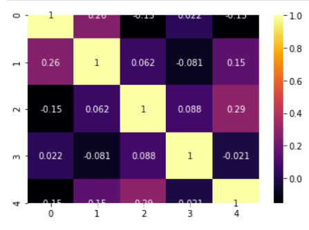
Correlation matrix, heatmap, covariance
We can build the correlation matrix right after ingesting the data. This matrix gives us an indication how much multicollinearity is present among the features/predictors.
Correlation matrix
model.ingest_data(X,y)
model.corrcoef()

>> array([[ 1.        ,  0.18424447, -0.00207883,  0.144186  ,  0.08678109],
       [ 0.18424447,  1.        , -0.08098705, -0.05782733,  0.19119872],
       [-0.00207883, -0.08098705,  1.        ,  0.03602977, -0.17560097],
       [ 0.144186  , -0.05782733,  0.03602977,  1.        ,  0.05216212],
       [ 0.08678109,  0.19119872, -0.17560097,  0.05216212,  1.        ]])
Covariance
model.covar()

>> array([[10.28752086,  1.51237819, -0.01770701,  1.47414685,  0.79121778],
       [ 1.51237819,  6.54969628, -0.5504233 , -0.47174359,  1.39094876],
       [-0.01770701, -0.5504233 ,  7.05247111,  0.30499622, -1.32560195],
       [ 1.47414685, -0.47174359,  0.30499622, 10.16072256,  0.47264283],
       [ 0.79121778,  1.39094876, -1.32560195,  0.47264283,  8.08036806]])
Correlation heatmap
model.corrplot(cmap='inferno',annot=True)
Statistical inference
Perform the F-test of overall significance
It retunrs the F-statistic and the p-value of the test.
If the p-value is a small number you can reject the Null hypothesis that all the regression coefficient is zero. That means a small p-value (generally < 0.01) indicates that the overall regression is statistically significant.
model.ftest()

>> (34.270912591948814, 2.3986657277649282e-12)
How about p-values, t-test statistics, and standard errors of the coefficients?
Standard errors and corresponding t-tests give us the p-values for each regression coefficient, which tells us whether that particular coefficient is statistically significant or not (based on the given data).
print("P-values:",model.pvalues())
print("t-test values:",model.tvalues())
print("Standard errors:",model.std_err())

>> P-values: [8.33674608e-01 3.27039586e-03 3.80572234e-05 2.59322037e-01 9.95094748e-11 2.82226752e-06]
   t-test values: [ 0.21161008  3.1641696  -4.73263963  1.14716519  9.18010412 -5.60342256]
   Standard errors: [5.69360847 0.47462621 0.59980706 0.56580141 0.47081187 0.5381103 ]
Confidence intervals
model.conf_int()

>> array([[-10.36597959,  12.77562953],
       [  0.53724132,   2.46635435],
       [ -4.05762528,  -1.61971606],
       [ -0.50077913,   1.79891449],
       [  3.36529718,   5.27890687],
       [ -4.10883113,  -1.92168771]])
Visual analysis of the residuals
Residual analysis is crucial to check the assumptions of a linear regression model. mlr helps you check those assumption easily by providing straight-forward visual analytis methods for the residuals.
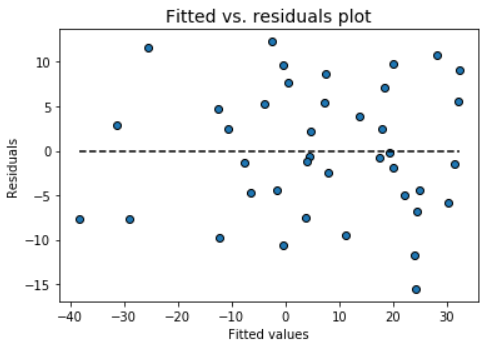
Fitted vs. residuals plot
Check the assumption of constant variance and uncorrelated features (independence) with this plot
model.fitted_vs_residual()
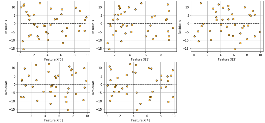
Fitted vs features plot
Check the assumption of linearity with this plot
model.fitted_vs_features()
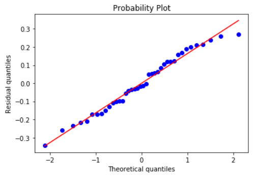
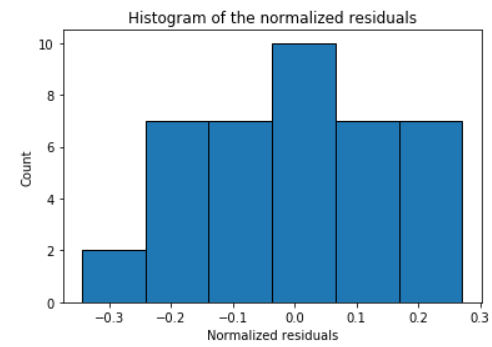
Histogram and Q-Q plot of standardized residuals
Check the normality assumption of the error terms using these plots,
model.histogram_resid()
model.qqplot_resid()