How regression metrics change with explanatory variables

Printing metrics as we add variables one by one

Let's say we define some random data using numpy as follows,

num_samples=40
num_dim = 5

X = 10*np.random.random(size=(num_samples,num_dim))
coeff = np.array([2,-3.5,1.2,4.1,-2.5])

y = np.dot(coeff,X.T)+10*np.random.randn(num_samples)
y = y.reshape(num_samples,1)

We can easily put them in a Pandas DataFrame as follows,

feature_cols = ['X'+str(i) for i in range(num_dim)]
target_col = ['y']
cols = feature_cols+target_col

df=pd.DataFrame(np.hstack((X,y)),columns=cols)

Now, if we check df, we will see something like this (the exact numbers will vary due to randomness),

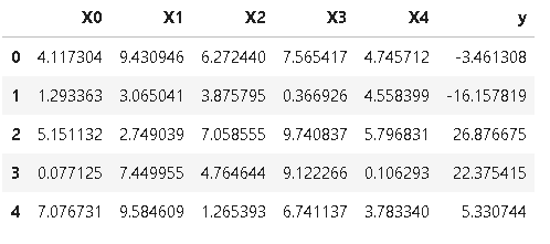
So, this problem has five explanatory variables - 'X0', 'X1', 'X2', 'X3', and 'X4'.

Now, we want to use mlr to check how the regression metrics change as we start with only one explanatory variable and gradually add more.

Simple code,

for i in range(1,6):
    m = mlr() # Model instance
    X = ['X'+str(j) for j in range(i)] # List of explanatory variables
    m.fit_dataframe(X=X,y='y',dataframe=df) # Fitting the dataframe by passing on the list
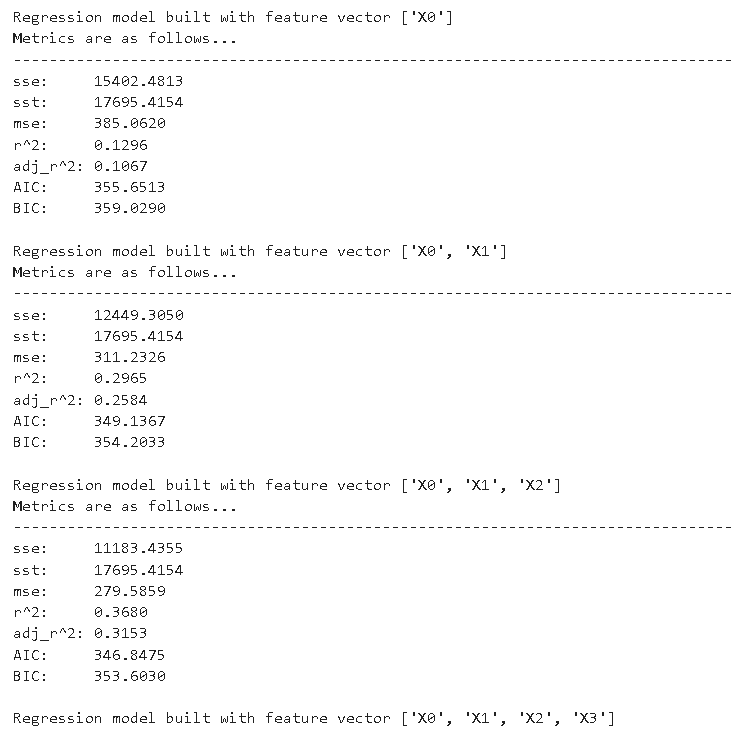
    print("\nRegression model built with feature vector", X)
    print("Metrics are as follows...")
    print("-"*80)
    m.print_metrics() # Printing the metrics

We should see something like following,

Plotting AIC/BIC as we add variables one by one

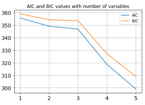
Let's say we want to plot the AIC and BIC values as the number of explanatory variables grow. Working with the same DataFrame df, following code plots the desired result,

# Two empty lists to hold the AIC and BIC
aic_lst=[]
bic_lst=[]

for i in range(1,6):
    m = mlr() # Model instance

    X = ['X'+str(j) for j in range(i)] # Create the list of explanatory variables
    m.fit_dataframe(X=X,y='y',dataframe=df) # Fit the dataframe

    # Call the methods and append to the lists
    aic_lst.append(m.aic())
    bic_lst.append(m.bic())

# Plotting code
plt.title("AIC and BIC values with number of variables")
plt.plot(np.arange(1,6),aic_lst)
plt.plot(np.arange(1,6),bic_lst)
plt.grid(True)
plt.legend(['AIC','BIC'])
plt.xticks([1,2,3,4,5],fontsize=14)
plt.yticks(fontsize=14)
plt.show()

Variables selection

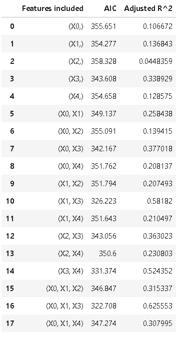
Often for small number of explanatory variables, we can scan through every possible combination of variables in the model and check their metrics - adjusted R^2 or AIC to see which model makes most sense from bias-variance trade-off point of view.

Following code accomplishes that by printing out a table of adjusted R^2 and AIC values for all combination of variable selection,

# Build a combinatorial list
from itertools import combinations
f=list(df.columns[:-2])
feature_list=[]
for i in range(1,6):
    feature_list+=list(combinations(f,i))

# Usual code of iterating over the list, model fitting, and storing the metrics
aic_lst=[]
adjusted_r2_lst=[]

for f in feature_list:
    m = mlr()
    X = list(f)
    m.fit_dataframe(X=X,y='y',dataframe=df)
    aic_lst.append(m.aic())
    adjusted_r2_lst.append(m.adj_r_squared())

metrics=(pd.DataFrame(data=[feature_list,aic_lst,adjusted_r2_lst])).T
metrics.columns=['Features included','AIC','Adjusted R^2']

The final table metrics should look something like,